Disclaimer & Copyright Notices; Optimized for the MS Internet Explorer

Trophic Terminology and Prediction

Research of the Organization for Economic Co-Operation and Development (OECD)

Soil & Water Conservation Society of Metro Halifax (SWCSMH)

Updated: August 12, 2015

(cf. Janus and Vollenweider, 1981; Mandaville, 2000; Soil & Water Conservation Society of Metro Halifax, 1991; and Vollenweider and Kerekes, 1982)

Sampling Frequency

In lakes with high storage capacity, sampling once a month per station and depth selected should provide an adequate picture of the average conditions; in some cases, and for some parameters, once every three months may be sufficient. On the other hand, lakes exhibiting high spatial and temporal variability, as well as lakes with an irregular flushing regime, may require more frequent sampling.

An absolute minimum sampling frequency of four times per year was recommended (winter, summer, spring, and autumn overturn) and a sampling frequency of at least once a month during periods of stratification. During the period of stratification, samples are essential from above and below the thermocline and from lower down in the hypolimnion. Samples from the hypolimnion very close to the lake bottom were particularly important. It was stressed that several sampling stations were required to describe conditions in lakes with complex morphometry, but if this was not possible, the minimum provision was that the lake should be sampled at the deepest point (or points). Only this minimum provision was followed in many cases and often a distorted picture of the average lake concentration resulted. Infrequent sampling usually gives a distorted picture of the resultant variables which have short-term variability and it is inadequate for the determination of peak values of chlorophyll a and daily primary production.

Depending on the conditions that exist in a water body, infrequent sampling might give adequate information for calculation of a mean value; this is true for most pristine oligotrophic lakes. It could, however, give a rather distorted picture in a highly eutrophic lake with a seasonally variable nutrient load.

Trophic Terminology

Fixed Boundary System or the Diagnostic Model:

In this system, a certain arbitrariness is unavoidable, and the danger exists that the respective categorization is rigidly applied. To avoid this, judgment about allocation of a given lake to a trophic category should not be based on only one or two parameters but on the total information.

The advantage of a fixed boundary system is its easy application by managers and technical personnel with only limited limnological training. In particular, it is apt to prevent gross misuse of the trophic terminology, which has often happened in the past.

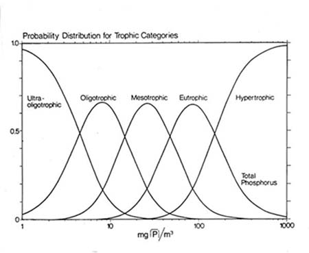
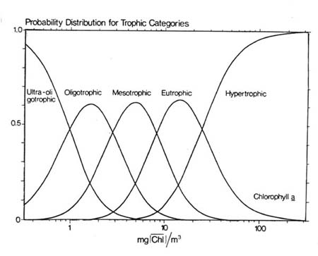
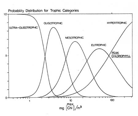
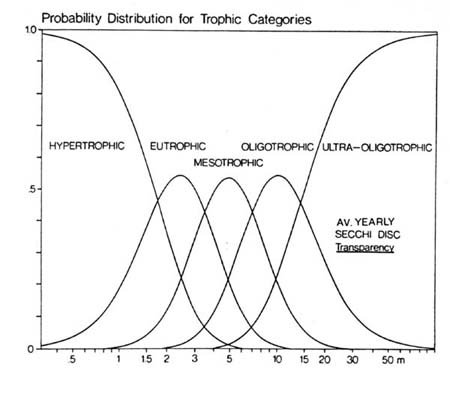
Table-2: Fixed Boundary System or the Diagnostic Model:

Trophic Category (Annual Mean Values)	[P]_λ	[chl]	[max. chl]	[Sec]^y	[min. Sec]^y
Trophic Category (Annual Mean Values)	mg/m³			m
Ultra-oligotrophic .....	≤ 4.0	≤ 1.0	≤ 2.5	≥ 12.0	≥ 6.0
Oligotrophic ...........	≤ 10.0	≤ 2.5	≤ 8.0	≥ 6.0	≥ 3.0
Mesotrophic .......	10 - 35	2.5 - 8	8 - 25	6 - 3	3 - 1.5
Eutrophic .......	35 - 100	8 - 25	25 - 75	3 - 1.5	1.5 - 0.7
Hypertrophic .......	≥ 100	≥ 25	≥ 75	≤ 1.5	≤ 0.7

Open Boundary System:

In contrast to the fixed boundary system, the open boundary system is more flexible in application, and "outliers" may be more easily realted to it.

The uncertainty in allocating a lake to a given category is taken into account and therefore, the probabilistic aspect becomes an important judgement element in predictive application of the system.In essence, it represents the qualified majority opinion of a large group of limnologists of how the trophic terminology is, and ought to be, applied in practice.

Accordingly, two lakes with numerically similar characteristics (which is always only one part of a qualitatively oriented judgement) may appear in different (though neighbouring) categories. However, as a rule it may be assumed that a gross error in allocation is made if more than one of the parameters used to define the trophic nature of a lake deviates by more than ą 2 standard deviations from the corresponding group means.

Table-3: Open Boundary System:

Variable (Annual Mean Values)		Oligotrophic	Mesotrophic	Eutrophic	Hypertrophic
Total Phosphorus mg/m³	x x ą 1 SD x ą 2 SD Range n	8.0 4.85 - 13.3 2.9 - 22.1 3.0 - 17.7 21	26.7 14.5 - 49 7.9 - 90.8 10.9 - 95.6 19	84.4 48 - 189 16.8 - 424 16.2 - 386 71	750 - 1200 2
Total Nitrogen mg/m³	x x ą 1 SD x ą 2 SD Range n	661 371 - 1180 208 - 2103 307 - 1630 11	753 485 - 1170 313 - 1816 361 - 1387 8	1875 861 - 4081 395 - 8913 393 - 6100 37
Chlorophyll a mg/m³	x x ą 1 SD x ą 2 SD Range n	1.7 0.8 - 3.4 0.4 - 7.1 0.3 - 4.5 22	4.7 3.0 - 7.4 1.9 - 11.6 3.0 - 11 16	14.3 6.7 - 31 3.1 - 66 2.7 - 78 70	100 - 150 2
Chlorophyll a Peak Value mg/m³	x x ą 1 SD x ą 2 SD Range n	4.2 2.6 - 7.6 1.5 - 13 1.3 - 10.6 16	16.1 8.9 - 29 4.9 - 52.5 4.9 - 49.5 12	42.6 16.9 - 107 6.7 - 270 9.5 - 275 46
Secchi Depth (m)	x x ą 1 SD x ą 2 SD Range n	9.9 5.9 - 16.5 3.6 - 27.5 5.4 - 28.3 13	4.2 2.4 - 7.4 1.4 - 13 1.5 - 8.1 20	2.45 1.5 - 4.0 0.9 - 6.7 0.8 - 7.0 70	0.4 - 0.5

Prediction

What emerged from the assessment of all information available, however, led to the conclusion that there is NO possibility of defining strict boundary values between trophic categories. Whilst the progression from oligo- to eutrophy is a gliding one- as has been stressed many times in literature- any one combination of trophic factors, in terms of trophic category allocation, can only be used in a probabilistic sense. Objective reasons exist for the uncertainty of classifying a given lake in different categories by two or more investigators, depending on the management of that body of water. It is strongly suggested that one refer to the probability distribution curves for the main components: average lake phosphorus (Figure-3), average (Figure-4) and peak chlorophyll a (Figure-5) concentrations and average yearly Secchi disc transparency (Figure-6).

Figure-3: Probability distribution curve for the average lake phosphorus:

Probability distribution curve for the average lake phosphorus

Figure-4: Probability distribution curve for the average chlorophyll a:

Probability distribution curve for the average chlorophyll a

Figure-5: Probability distribution curve for the peak chlorophyll a:

Probability distribution curve for the peak chlorophyll a

Figure-6: Probability distribution curve for the average yearly Secchi disk transparency:

Probability distribution curve for the average yearly Secchi disk transparency

Example of an application of the OECD Probability Distribution Diagrams for lakes in HRM, Nova Scotia:

Citation: Soil & Water Conservation Society of Metro Halifax. 1991. Limnological study of twenty seven Halifax Metro lakes. 136p.: ill., maps.

(Mandaville, S. M., and Shacklock, P. Based on our Stage-I protocol. Albro, Banook, Beaverbank, Bell, Bissett, Chocolate, First, Hubley Big, Kearney, Kinsac, Loon, Maynard, MicMac, Miller, Morris, Nicholson, Oathill, Papermill, Portuguese Cove, Rocky, Sandy [Bedford], Second, Settle, Springfield, Third, Tucker, and Williams [Halifax] lakes)

Since, the data of the 27 lakes below was only seasonal, i.e., three samples per year in most cases, peak chlorophyll a was not considered. One needs more extensive yearly data to confidently ascertain peak chlorophyll a.

[Img-probability-example-1]

We salute the Chebucto Community Net (CCN) of Halifax, Nova Scotia, Canada for hosting our web site, and we applaud its volunteers for their devotion in making `CCN' the best community net in the world